Flux mechanism in samurai - Hands-on samurai

In the previous practical session, we implemented a naive finite volume scheme for the inviscid Burgers equation using for_each_interval. We explained that this approach can be incorrect when dealing with fluxes at the interfaces between different levels in a multi-resolution mesh. To address this issue, we introduce the concept of fluxes and how to handle them correctly using samurai’s built-in flux mechanism. You will also see that the multi-dimensional case is handled in the same way.

How to start

If you have not already done so, activate the conda environment created in the Setup Instructions:

conda activate samurai-practical-session

For each step, we give you two main files, copy these two files into a new folder:

practical_session/material/step_name/CMakeLists.txt
practical_session/material/step_name/main.cpp

Then, create a build folder and compile the code as follows:

cmake -S . -B build
cmake --build build
cd build
./samurai_setup_test

We recommend changing the executable name in the CMakeLists.txt file to avoid confusion with the setup test and to keep track of your work at each step.

A comprehensive documentation about the flux mechanism in samurai is available at: finite volume schemes. We will provide a brief overview here.

samurai provides three types of schemes to handle fluxes in finite volume schemes:

the homogeneous linear scheme
the heterogeneous linear scheme
the nonlinear scheme

Following our example of the inviscid Burgers equation, we will focus on the nonlinear scheme in this practical session.

The definition of a nonlinear flux-based scheme requires defining a samurai::FluxDefinition<cfg> where the config in our case is:

using cfg = samurai::FluxConfig<samurai::SchemeType::NonLinear, stencil_size, field_t, field_t>;

We can observe that the scheme type is NonLinear. The stencil_size defines the number of neighboring cells used to compute the flux at a given cell interface. In our case, we will use a stencil size of 2, which means that the flux at the interface between cells i and i+1 will be computed using the values of u in cells i and i+1. The output field type and input field type are both field_t, which is the type of the solution field u. Note that the output field doesn’t always have the same number of components as the input field. For example, in the divergence operator, the input field is a vector and the output field is a scalar.

Now that the config is defined, we need to define the flux function for each Cartesian direction. In the scalar Burgers equation, the flux function is the same in each direction; only the cells change depending on the direction. To construct the flux in samurai, you have to build the following object:

samurai::FluxDefinition<cfg> burgers_flux(
        [&](samurai::FluxValue<cfg>& flux, const samurai::StencilData<cfg>& data, const samurai::StencilValues<cfg>& u)
        {
            // Compute flux at the interface using values in u
        });

auto scheme = make_flux_based_scheme(burgers_flux);

Let us explain the arguments of the lambda function:

flux: the output flux at the interface between two cells. You need to fill this value using the values of u.
data: contains information about the stencil, such as the indices of the cells in the stencil.
u: contains the values of the solution field u in the stencil cells.

A figure illustrating the stencil of size 2 for a 1D flux is given below:

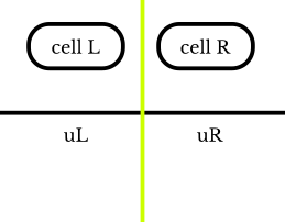
data will contain an array data.cells with two cell instances representing Cell L and Cell R, and an attribute data.cell_length containing the length of the cell. u will contain the values of the field in these cells: u[0] holds the left state (u_L), and u[1] holds the right state (u_R).

Note

Once you have implemented the flux-based scheme for the 1D Burgers equation, you can use it with lazy evaluation as follows:

auto conv = burgers_flux<decltype(un)>();

// in the time loop
unp1 = un - dt * conv(un);

This is given in the skeleton code provided in material/03-flux-burgers/main.cpp.

Exercise 5

Previously, the same flux is used in 1D and 2D, which means that the flux doesn’t depend on the direction. This is why we set the lambda function for the flux definition only once in the constructor. However, in general, the fluxes can differ across dimensions. To do that, we create a samurai::FluxDefinition<cfg> without parameters in the constructor and then set the flux function for each dimension separately:

samurai::FluxDefinition<cfg> my_flux;

my_flux[0].cons_flux_function = [](samurai::FluxValue<cfg>& flux, const samurai::StencilData<cfg>& data, const samurai::StencilValues<cfg>& u)
                           {
                               // flux in x-direction
                           };
my_flux[1].cons_flux_function = [](samurai::FluxValue<cfg>& flux, const samurai::StencilData<cfg>& data, const samurai::StencilValues<cfg>& u)
                           {
                               // flux in y-direction
                           };

Modify your implementation to create different flux functions for each dimension (x and y), even though they will be identical for this particular problem.

Write the 2D flux function in non-conservative form¶

In samurai, you can also define fluxes for non-conservative forms. This means you need to provide two fluxes at each interface in each direction: the flux going from left to right and the flux going from right to left in 1D. A conservative form can be seen as a particular case where the flux going from left to right is the negative of the flux going from right to left. You can find more information about this in the documentation on implementing a non-conservative scheme.

The syntax is the following:

samurai::FluxDefinition<cfg> my_flux;

my_flux[0].flux_function = [](samurai::FluxValuePair<cfg>& flux, const samurai::StencilData<cfg>& data, const samurai::StencilValues<cfg>& u)
                           {
                               flux[0] = ...; // left --> right (direction '+')
                               flux[1] = ...; // right --> left (direction '-')
                           };

Vector extension of the viscous Burgers equation¶

We will now consider the vector extension of the Burgers equation with a viscous term in its non-conservative form:

\mathbf{u}_t + (\mathbf{u}\cdot\nabla)\mathbf{u} = \nu \Delta \mathbf{u}, \qquad \mathbf{u}=(u,v).

(1)

Initial condition: Taylor-Green vortex¶

The Taylor-Green vortex is a well-known analytical solution of the incompressible Navier-Stokes equations, which can also be adapted for the viscous Burgers equation. The initial condition for the Taylor-Green vortex in 2D is given by:

\begin{aligned} u(x,y,0) &= -U_0\sin(kx) \cos(ky), \\ v(x,y,0) &= U_0\cos(kx) \sin(ky). \end{aligned}

(2)

where $U_0$ is the characteristic velocity and $k$ is the wave number. This initial condition represents a periodic vortex pattern. The domain is typically taken as the square $[0, 2\pi] \times [0, 2\pi]$ with periodic boundary conditions.

Convective operator¶

Let’s start with the convective part. The x-velocity at the interface is given by:

u_{I} = \frac{u_{L} + u_{R}}{2}.

(3)

The flux in the x-direction is computed using an upwind scheme. The formulas for the fluxes at the interface are:

F^x_{L \to R} = -u_{I} \frac{\text{sign}(u_{I}) - 1}{2} (\mathbf{u}_{R} - \mathbf{u}_{L}),

(4)

F^x_{R \to L} = u_{I} \frac{\text{sign}(u_{I}) + 1}{2} (\mathbf{u}_{R} - \mathbf{u}_{L}).

(5)

Diffusion operator¶

Now it’s time to implement the diffusion operator. We will use a linear homogeneous scheme, for which we need to create a new configuration:

using diff_cfg = samurai::FluxConfig<samurai::SchemeType::LinearHomogeneous, stencil_size, field_t, field_t>;

You can observe that the scheme type is now LinearHomogeneous.

The lambda signature changes because coefficients are returned. This allows samurai to build both explicit and implicit schemes. The flux definition changes slightly. Now, you need to define a lambda function with the following signature:

samurai::FluxDefinition<diff_cfg> diffusion_flux(
    [&](samurai::FluxStencilCoeffs<diff_cfg>& coeffs, double h)
    {
        // TODO: fill stencil interface coefficients
    });

For more details about implementing a linear homogeneous scheme, you can refer to the documentation on implementing a linear homogeneous scheme.

Conclusion¶

In this part, you have mastered samurai’s flux mechanism, a powerful tool that ensures conservation at multi-resolution interfaces. You learned to:

Configure and use nonlinear flux schemes for conservative formulations (scalar and vector Burgers)
Handle non-conservative formulations for coupled systems
Implement linear homogeneous schemes for diffusion operators
Combine multiple operators (convection + diffusion) in a single solver

The key advantage of samurai’s flux mechanism is its dimension-agnostic nature: the same flux definition works seamlessly in 1D, 2D, and 3D. You can also define different fluxes by dimension if needed. You also saw how to handle both scalar and vector fields with minimal code changes.

In the next part, you will apply these concepts to the Euler equations for compressible gas dynamics. This will require more sophisticated Riemann solvers (Rusanov, HLL, HLLC) and introduce new challenges such as custom boundary conditions and ensuring physical positivity. The flux mechanism you learned here will be the foundation for solving these complex multi-dimensional problems.

Hands-on samurai

Naive implementation of the Burgers equation

Hands-on samurai

Euler equations (part 1)